Walkthroughs
This article explains how to use Scanner by walking through a simple application: converting a video to grayscale.
Converting a video to grayscale
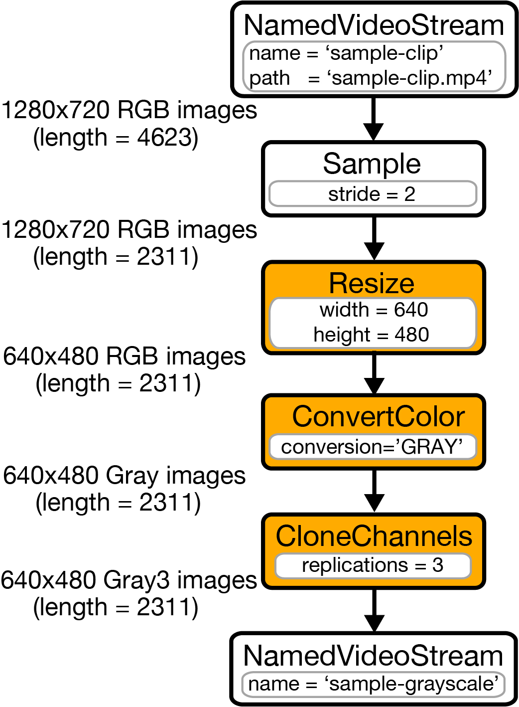
Let’s walk through a simple example that takes every other frame from a video, downsamples it, converts from color to grayscale, and then generates a new video from the transformed frames. The resulting application will look like the following sequence of operations:

To run the code for this example, first install Scanner (Installation). Then from the top-level Scanner directory, run:
cd /opt/scanner/examples/apps/walkthroughs
wget https://storage.googleapis.com/scanner-data/public/sample-clip.mp4
python3 grayscale_conversion.py
After grayscale_conversion.py exits, you should have a grayscale version of sample-clip.mp4 named sample-grayscale.mp4 in the current directory. Let’s see how that happened by looking inside main.py.
Starting up Scanner
The first step in any Scanner program is to create a Client object. The Client object manages your connection to the Scanner runtime and provides the API to execute new video processing jobs. By default, creating a client will first start an instance of Scanner on the local machine and then establish a connection to it:
import scannerpy as sp
import scannertools

sc = sp.Client()
Defining the Computation Graph
Scanner represents applications as computation graphs (Computation Graphs), with nodes that are Scanner operations (operations) and edges that represent streams of data. Scanner has built-in support for reading and writing videos, audio, lists of binary data, sequences of files, and SQL databases into and out of computation graphs. For example, let’s create a stream representing our video:
input_stream = sp.NamedVideoStream(sc, 'sample-clip', path='sample-clip.mp4')
NamedVideoStream is a stream that stores data in Scanner’s internal database format
(see Stored Streams for more detail). In this case, we stored the data under the name sample-clip for the video file sample-clip.mp4.
To implement the logic for downsampling all frames of a video to 640x480 and converting them to grayscale, we need to create a computation graph containing each of these operations. First, we’ll create an input operation that reads from our video:
frames = sc.io.Input([input_stream])
The frame object returned by the input operation represents the stream of frames in our video, and we’ll use it as the input to the next operation:
sampled_frames = sc.streams.Stride(frames, [2]) # Select every other frame
This Stride() operation selects only every other frame from the stream of frames we read from the video. (Stride comes from a special class of operations, called stream operations, that can subsample elements in stream. See Stream Operations.)
Next, we’ll resize the sampled frames by instantiating a Resize operation that will resize the frames in the sampled_frame stream to 640 x 480:
import scannertools.imgproc

resized_frames = sc.ops.Resize(frame=sampled_frames, width=[640], height=[480])
Resize returns a new stream of frames, which we call resized_frames. Resize is one of the collection of built-in operations in the standard_library. The built-in image processing operations, like Resize, live in the scannertools.imgproc module. (You can learn how to write your own operations by following the Tutorials.) Next, we will use another operation from the scannertools.imgproc module to convert the image to grayscale:
grayscale_frames = sc.ops.ConvertColor(frame=resized_frames, conversion=['COLOR_RGB2GRAY'])
To write a new video containing these grayscale frames, we are going to use Scanner’s builtin video compression functionality. However, video compression formats (such as h264) require three channels for each frame but our grayscale frames only have one channel. To rectify this, we’re going to define a new operation called CloneChannels that will allow us to produce a three channel frame by replicating our single channel grayscale image:
@sp.register_python_op()
def CloneChannels(config, frame: sp.FrameType) -> sp.FrameType:
    return np.dstack([frame for _ in range(config.args['replications'])])

grayscale3_frames = sc.ops.CloneChannels(frame=grayscale_frames, replications=3)
You can learn more about the syntax for defining new operations like CloneChannels by checking out the Operations guide. Finally, we write the frames to a new output stream called sample-grayscale by passing them into an output operation:
output_stream = sp.NamedVideoStream(sc, 'sample-grayscale')
output = sc.io.Output(resized, [output_stream])
Putting it all together, we have:
input_stream = sp.NamedVideoStream(sc, 'sample-clip', path='sample-clip.mp4')
frames = sc.io.Input([input_stream])
sampled_frames = sc.streams.Stride(frames, [2]) # Select every other frame
resized_frames = sc.ops.Resize(frame=sampled_frames, width=[640], height=[480]) # Resize input frame
grayscale_frames = sc.ops.ConvertColor(frame=resized_frames, conversion=['COLOR_RGB2GRAY'])
grayscale3_frames = sc.ops.CloneChannels(frame=grayscale_frames, replications=3)
output_stream = sp.NamedVideoStream(sc, 'sample-grayscale')
output = sc.io.Output(grayscale3_frames, [output_stream])
At this point, we have defined a graph that describes the computation to run, but we haven’t yet told Scanner to execute the graph.
Executing the computation graph
Executing a graph is done by calling run on the client object, specifying the outputs we want to produce:
sc.run(output, PerfParams.estimate())
This call will block until Scanner has finished processing the job. You should see a progress bar while Scanner is executing the computation graph. The PerfParams are parameters used to tune the performance of graph execution, e.g. the number of video frames that should be in memory at any one time. By default, the estimate() guesses an appropriate value of all parameters for your graph.
Exporting to mp4
Last, we can directly save our output stream as an mp4 file by calling save_mp4:
output_stream.save_mp4('resized-video')
After this call returns, an mp4 video should be saved to the current working directory called sample-grayscale.mp4 that consists of the grayscale frames that we generated. That’s the complete Scanner application!
Next Steps
To learn more about the features of Scanner, checkout the following:
Tutorials: introduces each of Scanner’s features with code examples.
Computation Graphs: describes how computation graphs are constructed and configured.
Operations: describes the capabilities of Scanner’s ops and how they work inside computation graphs.
Stored Streams: describes the stored stream interface.
Performance Profiling: describes how to profile Scanner applications and improve their performance.
Walking through a more advanced Jupyter-based app
To get a more detailed understanding of how Scanner can be used in a real application, we recommend trying the Jupyter notebook tutorial. To start the notebook, if you’re using Docker:
pip3 install --upgrade docker-compose
wget https://raw.githubusercontent.com/scanner-research/scanner/master/docker/docker-compose.yml
docker-compose up cpu
If you installed Scanner yourself, then run:
pip3 install jupyter requests matplotlib
cd path/to/scanner
jupyter notebook --ip=0.0.0.0 --port=8888
Then visit port 8888 on your server/localhost, click through to
examples/Walkthrough.ipynb, and follow the directions in the notebook.
